Aim to develop a predictive model to assess loan application risk accurately, leveraging applicant profiles, credit history, and loan details to evaluate their loan management potential. I will construct a binary classification model to differentiate 'good' loans from 'bad' ones.
Thanks for reading Ann’s Substack! Subscribe for free to receive new posts and support my work.
Utilizing the Loan Default Prediction Challenge dataset from Zindi, a platform championing data science solutions for African challenges, we accessed rich data curated to address local financial insights and predictive needs. The data we used for our model can be found as part of the Loan Default Prediction Challenge.
2. EDA(Exploratory Data Analysis)
1)Merge datasets
Our model's foundation was laid by integrating three distinct datasets, each offering unique insights into the client's profiles, loan performance, and historical loan interactions.
a) Demographic Dataset: This dataset provides a comprehensive overview of the client's demographic backgrounds, including personal identifiers, banking details, employment, and education levels, which are crucial for personalizing loan offerings.
● customerid: unique identification code (INT)
● birthdate: data of birth (STR)
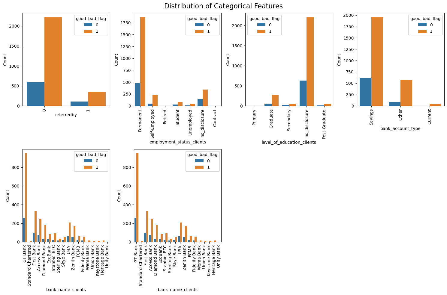
● bank_account_type: type of bank account (STR)
● longitude_gps: location (FLOAT)
● latitude_gps: location (FLOAT)
● bank_name_clients: name of bank (STR)
● bank_branch_clients: location of bank (STR)
● employment_status_clients: employment status of client (STR)
● level_of_education_clients: highest level of education of client (STR)
b) Performance Dataset: Central to our predictive model, this dataset encapsulates loan request specifics, including the vital good/bad loan indicator, serving as our model's target variable for predicting loan default risks.
● customerid: unique identification code (INT)
● systemloanid: id of the loan (INT)
● loannumber: number of loans (INT)
● approveddate: approval date of loan (STR)
● creationdate: creation date of loan (STR)
● loanamount: loan amount of loan (INT)
● totaldue: loan amount with interests and fees (INT)
● termdays: term of loan (INT)
● referredby: the customerid of the person who referred customer (INT)
● good_bad_flag: target variable (BOOL)
c) Historical Loan Dataset: Offering a window into past loan behaviours, this dataset enriches the model with patterns of previous loan applications and repayments, aiding in assessing clients' financial reliability.
● customerid: unique identification code (INT)
● systemloanid: id of the loan (INT)
● loannumber: number of loans (INT)
● approveddate: approval date of loan (STR)
● creationdate: creation date of loan (STR)
● loanamount: loan amount of loan (INT)
● totaldue: loan amount with interests and fees (INT)
● closeddate: date when loan was settled (STR)
● referredby: the customerid of the person who referred customer (INT)
● firstduedate: date of first payment due (STR)
● firstrepaiddate: actual date of first payment (STR)
Merging these datasets creates a multidimensional view of the clients, enabling a nuanced analysis pivotal for refining the loan approval algorithms.
2) Feature Engineering
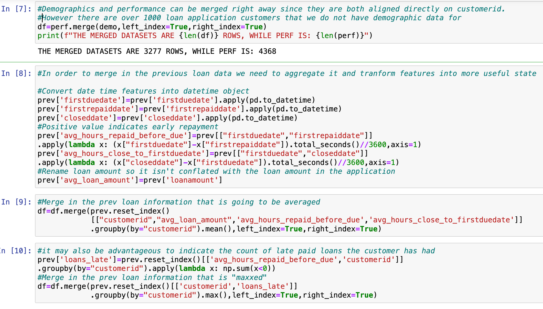
Some data was lost during the inner merge, approximately 18% after merging the demographics and performance data. Next, the previous loan data must be merged with the newly created dataset. This dataset contains multiple entries for each customer. Therefore, we had to transform the information into more valuable attributes through aggregation and feature engineering.
The previous loan dataset transformation/aggregation included the following:
● Conversion of date time features (‘firstduedate’, ‘firstrepaiddate’, and ‘closeddate’) into date-time objects
● Utilization of the new date-time objects to calculate the following:
1) average hours between the first due date and repaid date
2) average hours between the closed date and the first due date.
● These new attributes help determine whether a loan was repaid before it was first due.
● Renamed the ‘loanamount’ attribute to avoid confusion with the same ‘loanamount’ attribute in the performance dataset
● Averaged the loan amount, hours repaid before the due date, and hours between closed and first due date by the client to allow for a maximum one instance per client when merging with the other dataset
● Created a new attribute that calculates the number of loans that were paid late per client
4)Dealing with Missing values
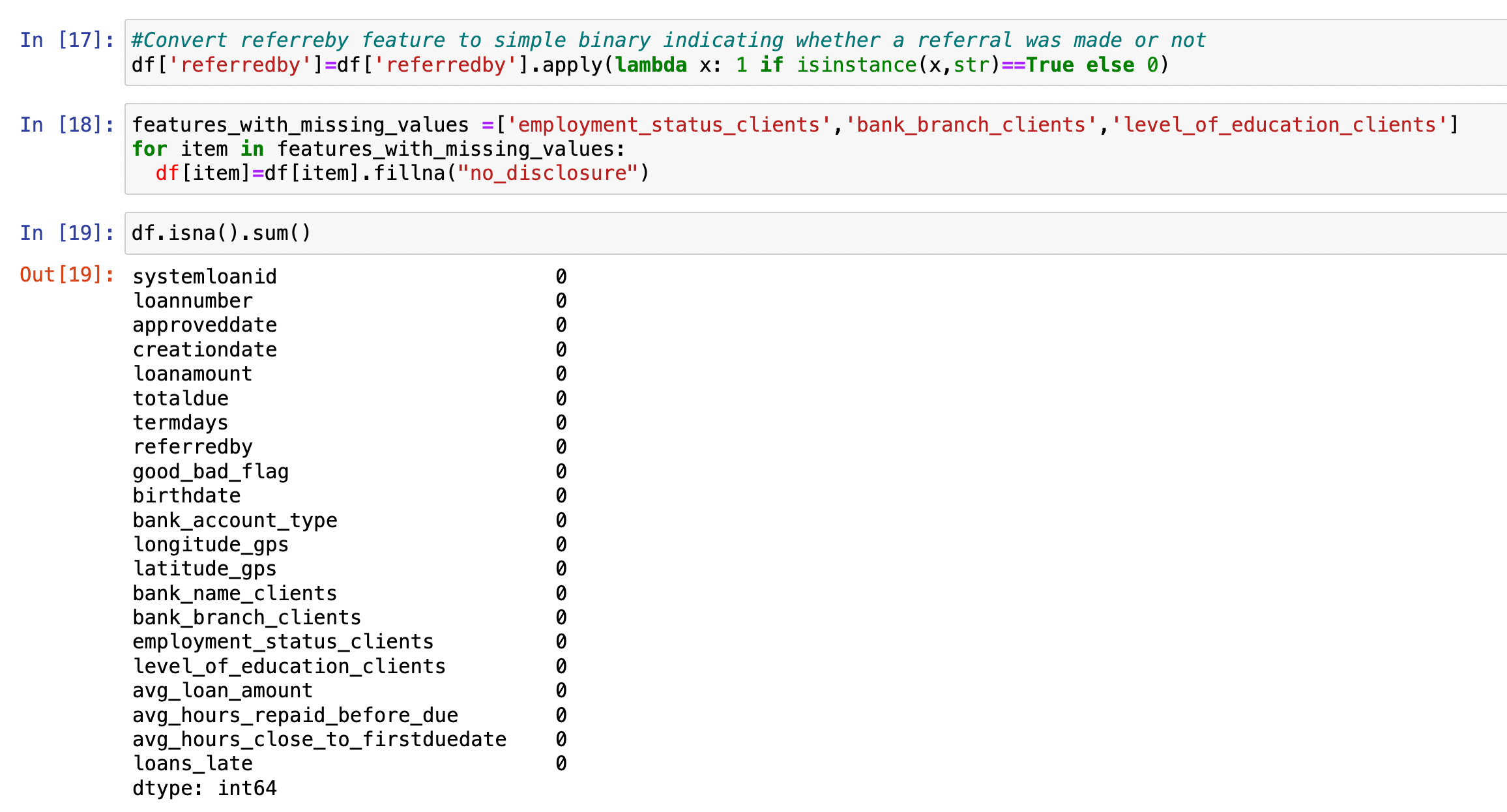
After merging all three datasets, some attributes contained missing values. Every attribute was critically analyzed, and a customized approach was used to deal with the missing values:
● For missing values in attributes 'employment_status_clients,' 'bank_branch_clients,' and 'level_of_education_clients' I decided to fill them in with a “no disclosure” label because they are likely relevant to the target variable about ‘good_and_bad flag. Also, it’s hard to identify an approach to estimate those values with the information provided confidently.
● For missing values in birth date, we converted the attribute to age and imputed using the mean.
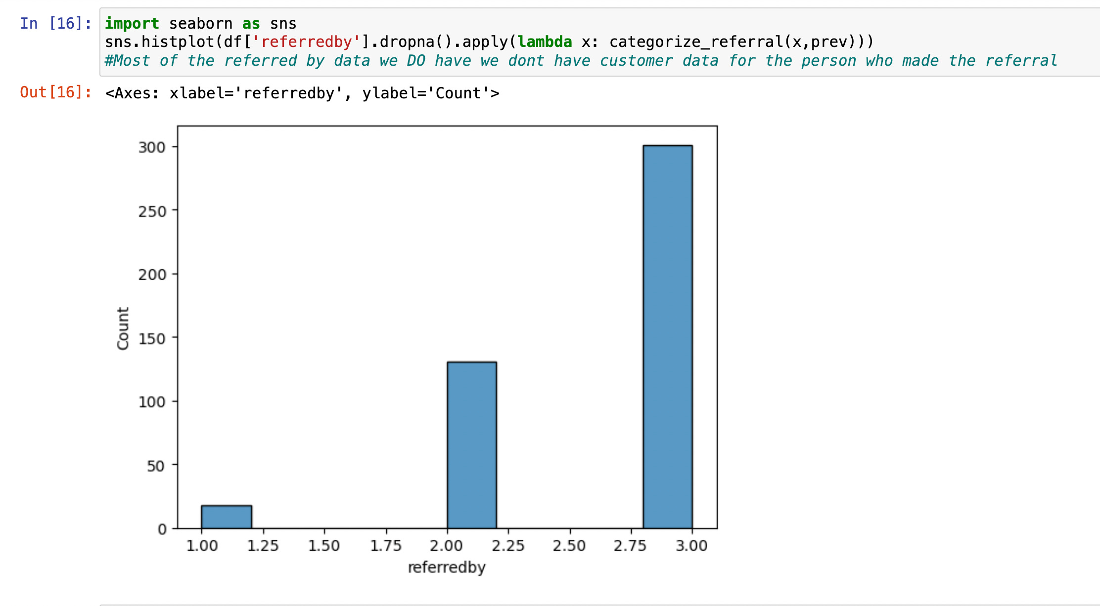
● For the missing values in the ‘referredby’ attribute. Initially, I would import additional information based on the ‘quality’ of the referral by looking up the referrer in the previous loan dataset. However, there was very little information on the referrers, so I converted it to a simple boolean variable, indicating whether someone referred the loan applicant. We then filled in the missing values with 0.
Next, some features- 'approveddate,' 'creationdate', 'bank_branch_clients' would likely not help predict the target variable. Therefore, we removed those columns.
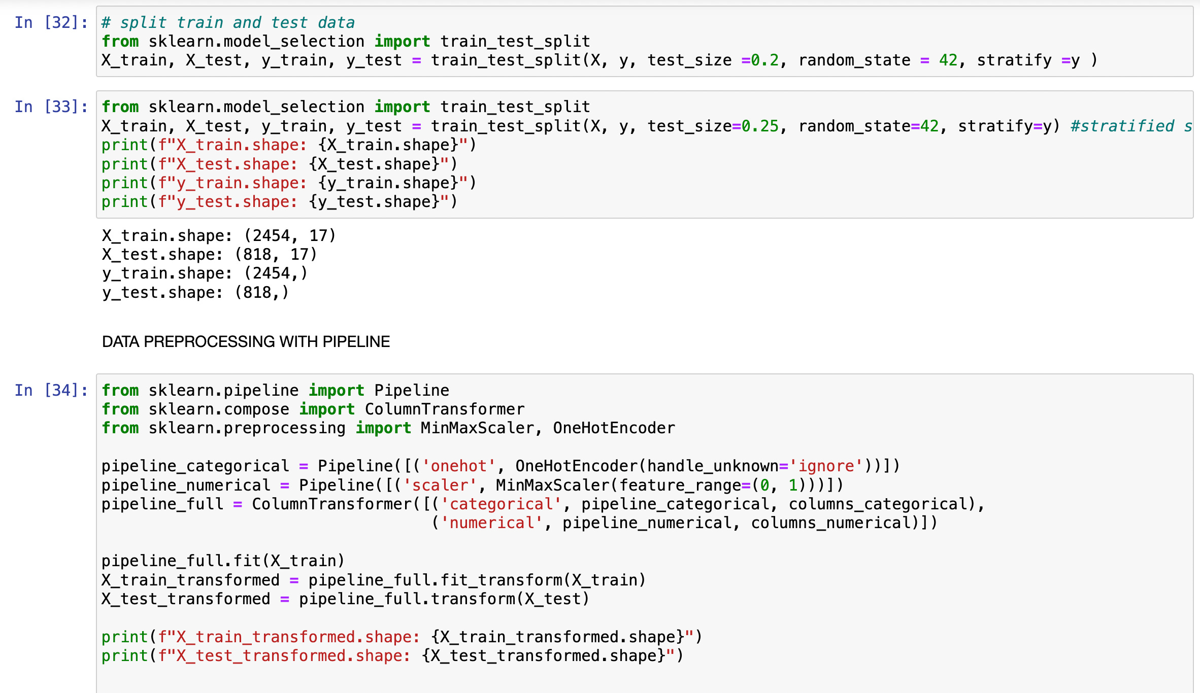
Finally, I divided all the remaining attributes into categorical and numerical variables to ensure the data was compatible with ingestion into a predictive model. A pipeline was created to apply one hot encoding to categorical variables and a MinMaxScaler to the numerical variables.
3. Modelling and Challenges
Handling missing values and integrating the three distinct datasets are challenging. Addressing these challenges demanded a meticulous approach involving comprehensive data exploration to analyze feature distributions.
Additionally, leveraging domain knowledge was essential to discern the relevance of different features for our model.
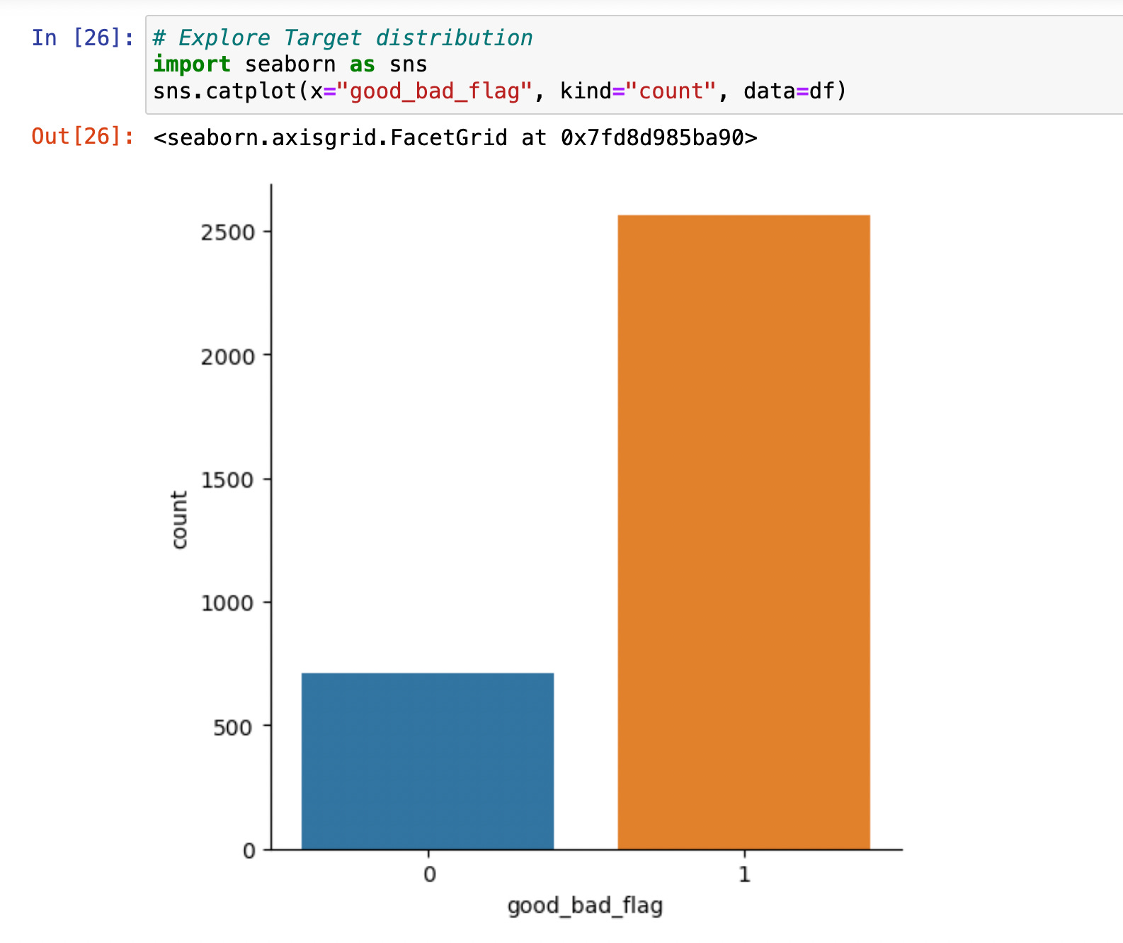
Besides, I identified an issue with dataset imbalance, as approximately 78% of the data were labelled as 'good.' In contrast, our objective was to accurately predict instances associated with the 'bad' flag denoting default payment. This necessitated employing techniques to address class imbalance and enhance the predictive capability of our model.
Model Design
1) Model Selection
To pick what models to use, I explored what our problem is. In this specific case, we are looking to tackle whether or not a client would default on a loan. From that, we would need to use a supervised machine-learning classification model.
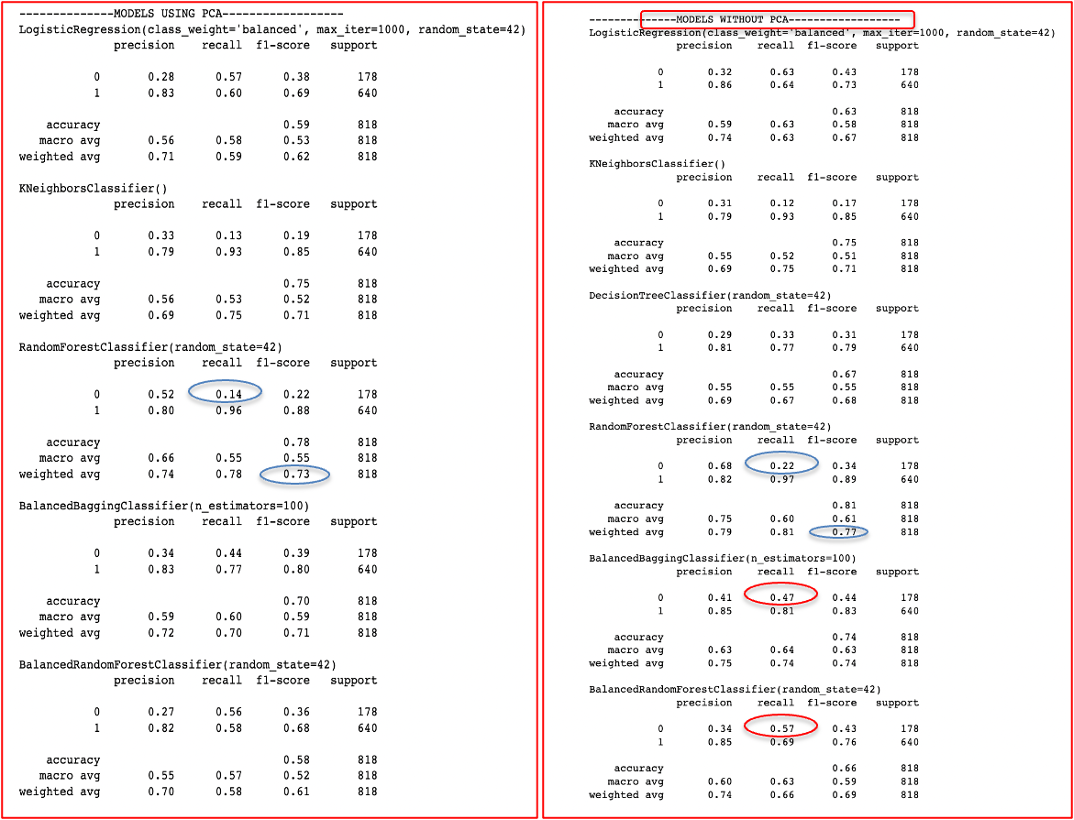
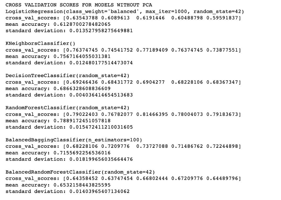
The following models were used for the data: LogisticRegression, KNeighborsClassifier, RandomForestClassifier, BalancedBaggingClassifier and BalancedRandomForestClassifier. I also tried using PCA(Principal Component Analysis) and without PCA to see how it would affect the accuracy scores. Due to our imbalanced data, we looked at the F1 score, recall, and precision to determine the best model. The following are detailed metrics:
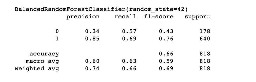
The information above shows that the RandomForestClassifier has a decent F1 score, but its recall and precision on the minority target population are abysmal. This is expected because of the imbalanced data set. The balanced models (BalancedBagging and BalancedRandomForest) have relatively lower F1 weighted averages but perform much better on predicting the minority target (recall of class 0 is 0.47 in the Balanced Bagging Classifier, and recall of class 0 is 0.57 in the BalancedRandomforest classifier). Therefore, I chose Balanced Random Forest as our best model without using PCA since I found that the model performs worse after using PCA.
2) Hyperparameter Tuning
Once we picked our model, we did some hyperparameter tuning. We tried GridSearch, RandomSearch and Optuna, and we ended up with RandomSearchCV, as it provides the highest weighted F1 score(0.72). However,. It is worth noting that the recall of class 0 dropped from 0.57 to 0.53 after hyperparameter tuning, although the weighted F1 score increased from 0.69 to 0.72. So we keep optimizing the model by looking at the importance of features.
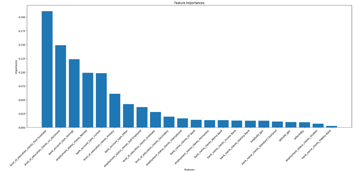
3) Feature Selection
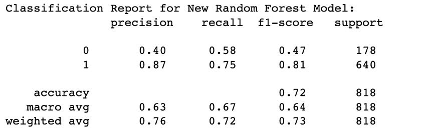
We strategically eliminated less significant features with importance scores below 0.002 through feature selection. This refinement yielded a substantial enhancement in the recall of class 0, escalating it from 0.53 to an impressive 0.58. This progress significantly bolsters our predictive capabilities for loan payment defaults. As a result, we've concluded that the BalancedRandomForest model, which employed the following feature selection, stands out as our final model.
4) Model Evaluation
We found that the ensemble models were the best performers, providing better accuracy, robustness, and generalization. Since we have an imbalanced dataset, we tried a Balanced Bagging Classifier and a Balanced Random Forest.
In terms of mean accuracy, the models rank as follows (from highest to lowest): Random Forest > KNN > Balanced Bagging Classifier > Balanced Random Forest Classifier > Logistic Regression.
Correctly identifying defaulting customers is a critical goal, so we want to prioritize recall of minority class 0, and weighted F1 score and AUC instead of mean accuracy. Additionally, iterative hyperparameter tuning and cross-referencing between methods like RandomSearch and Optuna is a solid strategy for achieving better model performance. By comparing the
recall of class 0 of RandomSearch and Optuna, we found that RandomSearch outperformed Optuna.
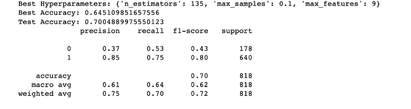
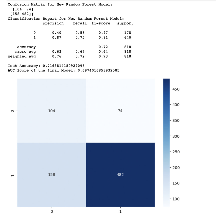
Below is the final metrics after RandomSearch hyperparameter tuning and feature selection:
Best Hyperparameters: {'n_estimators': 135, 'max_samples': 0.1, 'max_features': 9}
Recall improved to 0.59 for the minority class and 0.70 for the majority class. This indicates that the model accurately identifies around 59% of actual defaulting instances, surpassing random guessing.
Precision: class 0 precision is 0.40, and for class 1, it's 0.87. This indicates that when the model predicts class 0, it's correct 40% of the time, and when it predicts class 1, it's correct 87% of the time.
Our model seems to have relatively high precision and recall for class 1 (non-defaulting customers), indicating that it's good at predicting non-defaults.However, the recall for class 0 (defaulting customers) is lower, suggesting that the model struggles to identify defaults.
Attempts were made to mitigate the data imbalance using the SMOTE technique, yet the improvements were modest.
The weighted avg. F1-score of 0.73 indicates a balanced performance between precision and recall for the overall dataset. To correctly identify defaulting customers is crucial, we might need to continue improving the model's recall for class 0, even if it means sacrificing some precision. We could also consider adjusting the model's decision threshold to achieve a better trade-off between precision and recall.
Weighted Avg: The weighted average precision is 0.76, weighted average recall is 0.72, and weighted average F1-score is 0.73.
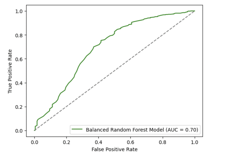
AUC of 0.70 suggests that the model has some discriminatory power, but it might not be very strong. In other words, the model is somewhat better than random guessing but might not be able to perfectly separate the two classes. This suggests there is significant room for further enhancement in order to optimally predict loan defaults, a critical aspect in mitigating financial risks and optimizing decision-making processes.
4. Conclusions
1) Is the model helpful?
Through rigorous exploration of the dataset and the application of various machine learning models, we successfully created a model with the potential to address the challenge. The chosen BalancedRandomForestClassifier, supported by RandomSearch hyperparameter tuning and feature selection, demonstrated improved performance in predicting loan defaults. While the model can only predict 58% of default payments, it does offer a moderate solution that could be further refined to enhance predictive accuracy with more work.
2) What can we learn from the dataset?
The dataset provided valuable insights into the attributes and factors affecting loan default predictions. Merging multiple datasets and performing feature engineering unveiled meaningful relationships between client demographics, loan details, and repayment behaviour. Missing value handling, strategic feature selection, and consideration of imbalanced class distributions were critical steps in enhancing model performance. We also observed the importance of continuous iteration, evaluation, and experimentation to refine the model's predictive capabilities.
3) What would we do next to improve the model?
To further enhance the model's predictive accuracy for loan defaults, the following steps could be considered:
● Feature Engineering: Explore additional features that might provide insights into loan repayment behaviour. These features could include financial indicators, socio-economic factors, and external economic trends impacting loan defaults.
● Advanced Techniques for Imbalanced Data: Experiment with more advanced techniques for addressing class imbalance, such as combining under-sampling and over-sampling methods, and exploring more complex algorithms designed for imbalanced datasets.
● Model Ensemble Strategies: Investigate ensemble techniques that combine the predictions of multiple models. Ensemble methods like stacking and boosting could potentially improve overall performance by leveraging the strengths of individual models.
● Threshold Adjustment: Experiment with adjusting the decision threshold of the model. By tuning the threshold, we can achieve a better trade-off between precision and recall, which is particularly important for classifying loan defaults.
● Interpretability and Explainability: Invest in techniques to make the model more interpretable and explainable. This will not only help in understanding model predictions but also gain the trust of stakeholders.
By addressing these aspects and incorporating cutting-edge methodologies, the model's accuracy and predictive power can be further improved, ultimately contributing to more effective loan default predictions and risk management
Thanks for reading Ann’s Substack! Subscribe for free to receive new posts and support my work.